Data engineering · 18 min read
What a fire leaves behind
A thermal satellite sees a fire while it burns. Sentinel-2 sees the scar afterwards, in light the eye cannot register. This is how I turn that into burn severity per 2 km cell, and why the machine learning model I trained is not allowed to overrule the arithmetic it sits next to.
This is the second pipeline in Space Insights. The first one, described here, watches the whole planet for heat. This one watches four regions for damage. They are built to disagree with each other, which is the point.
Two satellites, two different questions
A VIIRS thermal detection means: at the moment this satellite passed overhead, this 375 m pixel was radiating more energy than its surroundings. That is a statement about an instant. If the fire started after the overpass and burned out before the next one, VIIRS never saw it. If the sky was clear and the fire was hot, it did.
Sentinel-2 asks something else entirely: on the next cloud-free pass, how much living vegetation is still here compared to last time? That is a statement about a consequence. It cannot tell you when the fire happened or how hot it burned. It can tell you that four square kilometres of canopy that existed nine days ago are now char.
Neither is a better version of the other. The interesting engineering is in building both and then joining them.
Why the difference, and not the reflectance
Sentinel-2 carries thirteen spectral bands. Burn detection needs three of them, plus a fourth for housekeeping.
| Index | Bands | What it keys on |
|---|---|---|
NDVI | B08 (842 nm) - B04 (665 nm) | Chlorophyll absorbs red light; leaf structure scatters near-infrared. High values mean green, living plants. |
NBR | B08 (842 nm) - B12 (2190 nm) | Healthy leaves are bright in near-infrared and dark in shortwave infrared, because leaf water absorbs there. Fire destroys the structure and drives out the water: NIR collapses, SWIR rises. |
Both are normalised differences, (a - b) / (a + b), which keeps them bounded and cancels out most illumination effects. Healthy canopy sits at high positive NBR. A fresh burn scar sits near zero or below.
Here is the trap. It is tempting to declare a threshold on NBR itself and call anything below it burnt. That does not work, and the reason is worth stating precisely: low NBR is not evidence of fire. Bare rock has low NBR. So does a ploughed field, a sand dune, a quarry, a road, and a scar from three summers ago. An absolute threshold flags all of them forever.
So the pipeline never asks what a place looks like. It asks what changed:
def dnbr(nbr_pre: FloatArray, nbr_post: FloatArray) -> FloatArray:
    """Delta NBR between a pre-fire and a post-fire observation.

    Positive values indicate vegetation loss; > 0.27 is commonly treated as
    moderate-to-high burn severity (USGS/FIREMON thresholds).
    """
    return np.asarray(nbr_pre, dtype=np.float64) - np.asarray(nbr_post, dtype=np.float64)
One subtraction, and the entire land-cover problem disappears. Differencing the same ground against itself means the baseline cancels: whatever that patch was, a drop of 0.5 says it just lost most of its living biomass. The quarry stays a quarry and never appears.
The cost of differencing
Reading pixels without downloading scenes
The ingest runs on GitHub Actions rather than inside Databricks, for the same reason the FIRMS one does: Free Edition restricts serverless outbound traffic to an allowlist, and Copernicus is not on it. A scheduled job outside the lakehouse reaches the open internet and pushes inward. I call it a ground station and there are two of them.
That placement creates the real constraint. A single Sentinel-2 tile is roughly a gigabyte. A monitored region is a 60 km box, a small fraction of one tile, and there are four of them, every day. Downloading scenes and cropping them locally would move hundreds of gigabytes a month through a shared CI runner to extract a few megabytes of signal.
It is also unnecessary, because the assets are cloud-optimised GeoTIFFs. A COG is internally tiled with a header that says which byte ranges hold which tiles, so a reader that knows what it wants can issue HTTP range requests for exactly those bytes:
def read_window(href: str, bbox_wgs84: BoundingBox) -> RasterWindow:
    """Read the pixels covering `bbox_wgs84` from an s3:// asset at native resolution."""
    vsipath = "/vsis3/" + href.removeprefix("s3://")

    with rasterio.Env(**_GDAL_OPTIONS), rasterio.open(vsipath) as src:
        bounds = transform_bounds("EPSG:4326", src.crs, *bbox_wgs84.as_tuple())
        window = from_bounds(*bounds, transform=src.transform)
        window = window.round_offsets().round_lengths()
        data = src.read(1, window=window, boundless=True, fill_value=0)
        return RasterWindow(
            data=data,
            transform=src.window_transform(window),
            crs=str(src.crs),
            nodata=src.nodata,
        )
Three details in there each cost me time to learn:
- Reproject the bounds, not the pixels. The region is defined in latitude and longitude; the scene is in a UTM zone. Converting the corners into the scene's coordinate system means the read happens in native pixel space with no resampling at all. Reprojecting afterwards, once, is both faster and less lossy than resampling on read.
GDAL_DISABLE_READDIR_ON_OPEN=EMPTY_DIR. Without it, GDAL lists the entire containing prefix every time it opens a file. On object storage that listing costs more than the pixel read it is preparing for.- Boundless reads with a fill value. When a region runs off the edge of a tile, the read is padded rather than clipped, so every band patch comes back the same shape and stays alignable. The padding is zero, which I have to remember to treat as invalid later, perfectly dark, perfectly plausible ground that was never observed.
One more wrinkle: Copernicus storage speaks the S3 protocol but is not AWS, and GDAL will only take the credentials as real process environment variables: rasterio.Env() refuses AWS_* credential options passed directly. Path-style addressing, custom endpoint, and a region string that means nothing. Half an hour of confusion, one comment in the codebase so nobody repeats it.
Landing it, and the commit marker
Each band patch becomes a compressed GeoTIFF in a Unity Catalog volume, with a metadata row in Delta. The write order is deliberate:
io.execute(*bronze.delete_patches_statement(catalog, spec.name, scene.scene_id))
io.execute(*bronze.delete_scene_statement(catalog, spec.name, scene.scene_id))
for band, href in scene.assets.items():
    raster = cdse.read_window(href, patch_bbox)
    volume_path = patches.patch_volume_path(catalog, spec.name, scene.scene_id, band)
    io.upload(volume_path, patches.to_geotiff_bytes(raster))
    io.execute(*bronze.insert_patch_statement(...))
io.execute(*bronze.insert_scene_statement(catalog, spec.name, scene))
The scenes row goes last, and it is the commit marker. If the run dies after two of four bands, there are orphan files and orphan index rows but no scene row, so the next run treats that scene as never ingested, deletes the debris, and redoes it. Written first, the scene would look complete while missing the bands that make it usable, and the transform would happily compute indices from whatever landed. Same trick as a write-ahead log, and it costs nothing but ordering.
From pixels to cells
Inside the lakehouse, patches become per-cell numbers. Four steps, each with one decision in it.
Align the bands. Red and near-infrared are 10 m; shortwave infrared and the classification band are 20 m. Everything is resampled onto the shortwave grid, because NBR is the point and averaging down loses less than upsampling would invent. The classification band uses nearest-neighbour rather than averaging: the mean of "cloud" and "vegetation" is not a category.
Mask what cannot be trusted. Sentinel-2 ships a Scene Classification Layer, and seven of its classes are unusable:
# Sentinel-2 L2A scene classification (SCL) classes that are unusable for
# burn detection: no data, saturated, cloud shadow, cloud medium/high
# probability, thin cirrus, snow/ice.
INVALID_SCL_CLASSES = frozenset({0, 1, 3, 8, 9, 10, 11})
Cloud shadow, class 3, is the one that matters most and it is not obvious. Cloud is easy: it is bright, it is white, and it produces nonsense in every band at once. A shadow is subtle and it is directional: it suppresses near-infrared much more than shortwave infrared, which is precisely the asymmetry a fire produces. An unmasked shadow does not add noise, it forges the signal. It was the single largest source of false detections before I handled it.
Convert to reflectance. Since processing baseline 04.00 the stored integers carry an offset, so the conversion is (DN - 1000) / 10000. Miss the offset and every index in the pipeline is quietly biased in the same direction, the kind of bug that produces plausible, consistent, wrong numbers.
Average onto the grid. This one has a trick I am fond of:
# avg(x * valid) / avg(valid) = masked mean; avg(valid) = valid fraction.
cell_valid = _to_grid(valid_float, swir, grid)
cell_ndvi = _to_grid(np.where(valid, ndvi, 0.0), swir, grid) / cell_valid
cell_nbr = _to_grid(np.where(valid, nbr, 0.0), swir, grid) / cell_valid
Average-reprojection is linear, so averaging value x mask and dividing by the average of the mask gives exactly the cloud-free mean of the cell. And the denominator is not scaffolding; it is the fraction of the cell that was actually visible. One reprojection produces both the measurement and its own quality metric, for free. That quality metric travels all the way to the model.
The grid, and a bounding box I can never move
Cells are a fixed 0.02 degree lattice (about 2.2 km) anchored at each region's north-west corner, with IDs like r014c007. Central Portugal is 30 by 30.
Frozen by construction
Degree-based cells are also anisotropic with latitude. At 62°N in the Northwest Territories region, 0.02° of longitude is about a kilometre while 0.02° of latitude is still 2.2 km. This is exactly the projection problem I solved with hexagons on the other pipeline, and I deliberately did not solve it that way here: these cells are reprojection targets, and averaging pixels onto them needs an affine transform, which H3 cells do not have. I widened the box instead and kept comparisons inside a region rather than across.
Regions chosen by the other pipeline
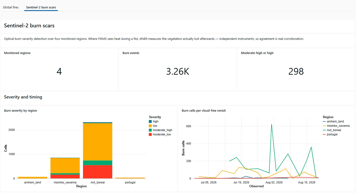
Three of the four monitored regions were picked by querying the fires globe: the largest active clusters on a particular morning in July, across deliberately different biomes: boreal spruce in Canada, miombo woodland on the Angola/DRC border, tropical savanna in Arnhem Land, plus Mediterranean pine in Portugal. dNBR behaves differently in each. One pipeline finds where the planet is burning; the other goes and measures the scars.
The delta, in one window function
Two dbt models carry the whole detection. First, collapse to one observation per cell per day, weighted by how much of the cell each scene actually saw, and throw away anything below 30% visible. Then:
lag(nbr) over (partition by aoi, cell_id order by sensed_date)         as nbr_pre,
lag(sensed_date) over (partition by aoi, cell_id order by sensed_date) as date_pre
...
nbr_pre - nbr                      as dnbr,
datediff(sensed_date, date_pre)    as days_between
Every row is a revisit pair: this clear observation against the previous clear observation of the same ground. days_between is carried along because the pairing is over clear observations, not calendar days (sometimes five, sometimes twenty-five after a cloudy fortnight) and anyone who ignores that will read autumn as fire.
The quality gate belongs upstream of this, in the daily model, and that placement is not arbitrary. A cell with 12% valid pixels produces a number computed from a handful of surviving pixels: real, but not a measurement. Dropping it means a clouded pass produces no observation rather than a bad one, which matters here specifically, because this window function pairs consecutive observations, so one bad value would poison two deltas rather than one.
Then the detector, which is arithmetic and a citation:
case
    when dnbr >= 0.66 then 'high'
    when dnbr >= 0.44 then 'moderate_high'
    when dnbr >= 0.27 then 'moderate_low'
    else 'low'
end          as severity
from dnbr_deltas
where dnbr >= 0.10
  and days_between <= 30
Those breakpoints are the published USGS/FIREMON severity classes, applied unmodified. No fitted parameters, no training data, nothing to retrain, and anyone who knows the literature can audit the whole detector in ten seconds. The 30-day guard is what stops slow seasonal drying from being read as fire.
Then why train a model at all
Because a threshold asks a one-dimensional question, and the data has five dimensions. Consider two rows the pipeline actually produces:
| dnbr | nbr_post | ndvi | days | visible | |
|---|---|---|---|---|---|
| A | 0.50 | 0.38 | 0.55 | 27 | 42% |
| B | 0.50 | -0.15 | 0.11 | 5 | 95% |
The rule classifies both as moderate_high, because it can only see the first column. But A is a poorly-observed cell that drifted over four weeks and still has living vegetation on it: harvest, drought stress, or shadow that survived the mask. B lost half its reflectance ratio in five days, ended up below zero, and its vegetation index collapsed at the same time, all on a cleanly observed cell. Only B looks like fire.
Distinguishing them requires looking at all five columns jointly, which is a different kind of question than any threshold can answer. So:
FEATURE_COLUMNS = ["dnbr", "nbr_post", "ndvi", "days_between", "valid_fraction"]

# Expected share of anomalous revisit pairs; drives the IsolationForest
# decision threshold. Kept explicit so it's logged with every training run.
CONTAMINATION = 0.01


def make_model(random_state: int = 42) -> Pipeline:
    return Pipeline([
        ("scaler", StandardScaler()),
        ("forest", IsolationForest(
            n_estimators=200,
            contamination=CONTAMINATION,
            random_state=random_state,
        )),
    ])
Unsupervised, because there is no truth to supervise with
Nobody hands you a per-cell, per-date burnt-or-not label for central Portugal. I could hand-label some, but I would be labelling by looking at dNBR, which means training a model to reproduce the thresholds it is supposed to be independent of. That is not validation, it is laundering.
So the model learns what normal looks like from the overwhelming majority of rows where nothing happened, and scores everything by how far it sits from that. IsolationForest suits the shape of this problem specifically: it needs no distance metric or density estimate over mixed-scale features, it trains in seconds on the tens of thousands of rows this pipeline accumulates, and its contamination parameter maps onto a claim I can actually defend out loud, about one in a hundred revisit pairs is unusual.
Two small choices in that pipeline are worth naming. The scaler is inside the estimator rather than applied beforehand: tree splits do not need it, but bundling it means the registered artifact is self-contained and inference cannot forget a preprocessing step that training applied, because there is no separate step to forget. And the seed is fixed, so retraining changes the champion when the data changed, not when the random number generator did.
The two features that are not about fire
Three of the five inputs are what you would expect: the delta, the absolute state it landed in, and an independent vegetation index from a different band pair as corroboration. If NBR fell but NDVI is untouched, something other than combustion happened.
The other two are the interesting ones, and I think they are the single best decision in this model:
| Feature | What it actually encodes |
|---|---|
days_between | How long since the last clear view. A 0.4 drop over five days is dramatic; the same drop over twenty-eight days is a season changing. |
valid_fraction | How much of the cell was genuinely visible. A large delta on a 35%-visible cell is far more likely to be residual cloud than fire. |
Neither is a property of the fire. Both are properties of how the measurement was taken, and feeding them in is what lets the model learn that a big delta over a long gap, or on a barely-observed cell, is ordinary rather than alarming. That is exactly the false-positive population a threshold structurally cannot suppress, because a threshold has no idea how its input was produced.
Including measurement provenance as model input is unusual enough that it deserves its stated risk: the model can learn to distrust all long-gap observations, including real ones. With the rule already bounding events at 30 days, I am comfortable with that bias today, and it is the first thing I would re-examine once I have ground truth.
What I log, having no accuracy to report
mlflow.log_metrics(
    {
        "training_rows": float(len(features_df)),
        "anomaly_rate": float(flags.mean()),
        "score_p99": float(scores.max() if len(scores) else 0.0),
    }
    | {f"training_rows_{aoi}": float(n) for aoi, n in aoi_counts.items()}
)
There is no precision or recall here and I decline to invent any. What these three do tell me: anomaly_rate should land near the contamination parameter, which is the sanity check that the fit is not degenerate; score_p99 tracks how extreme the tail is between runs; and the per-region row counts reveal whether one area has quietly come to dominate training, which is the most likely way this model goes wrong as regions are added.
The region is used for those counts and then dropped; it is not a feature. One model spans all four biomes, which is a real tradeoff. Per-region models would capture local baselines better, but with four regions and a few months of history they would mostly capture noise, and a newly added region would have no model at all until it accumulated its own history. Pooling buys a cold-start answer and a single champion to reason about. It stops being the right call when any one region has enough revisits to stand alone.
Below a hundred rows the job refuses to train, with a message saying what to do about it. IsolationForest will cheerfully fit twenty rows and produce confident nonsense; a loud failure is much cheaper than a quiet one.
The model is not allowed to overrule the rule
Both detectors write to gold, separately, and both reach the map. The rendering is where the relationship becomes visible to a person:
color:     cell.is_anomaly ? "#f43f5e" : severityColor(cell.dnbr),
weight:    cell.cell_id === selectedCell ? 3 : cell.is_anomaly ? 2 : 0.5,
fillColor: severityColor(cell.dnbr),
The fill is always the measurement. The outline is the model. It draws around cells it finds unusual, and it never repaints one. A user always sees what was physically measured, with the model's opinion as an annotation on top, and the two are allowed to visibly disagree, which is the entire reason to run both.
That principle shows up operationally too:
except mlflow.exceptions.MlflowException as e:
    # A fresh environment has data before its first training run - skip
    # scoring rather than failing the whole transform DAG.
    logger.warning("No champion model for %s yet; skipping scoring", model_name, exc_info=e)
    return 0
A new environment has data flowing before anyone has trained anything. Failing the whole daily pipeline over that would be wrong: the physics-based tables are complete and correct, and only the optional enrichment is missing. The pipeline degrades to the rule instead of going down. That is only possible because the rule was never a placeholder for the model.
One more deliberate choice: scored rows are never rewritten. Each carries the model version that produced it, and promoting a new champion does not retroactively change history. The table records what the system believed when it believed it, which is what makes the version column mean anything. The cost is that adjacent dates on the map can carry scores from two different models. I would rather have that than an unfalsifiable, always-current opinion.
Checking one pipeline against the other
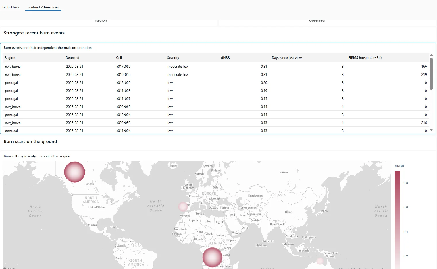
The payoff for building both. A view maps thermal detections onto this pipeline's analysis grid and matches them to burn-scar observations within three days. What makes the agreement worth anything is how little the two measurements share:
| Thermal (FIRMS) | Optical (Sentinel-2) | |
|---|---|---|
| Phenomenon | Emission while burning | Reflectance change after burning |
| Spectrum | Mid and thermal infrared | Near and shortwave infrared |
| Platform | VIIRS on three polar orbiters | Sentinel-2 A and B |
| Timing | During the fire | On the next clear pass |
| Blind to | Fires between overpasses | Anything under cloud |
Different physics, different instruments, different satellites, different failure modes. Where both fire, that is genuine corroboration rather than one measurement counted twice, and the three-day window exists precisely because the scar is observed after the heat.
What I would change
The join is duplicated logic. That cross-validation view recomputes my grid cell IDs in SQL, reimplementing a formula that lives in Python. Nothing enforces that the two stay in sync. Change the grid and the view produces wrong joins silently instead of failing. A shared fixture asserting both implementations agree is the real fix; a comment is what is there today.
The model is unvalidated, and I say so. Not weakly validated - unvalidated, in the sense that no external ground truth has ever been compared against it. The fix is not a better model, it is data: the European Forest Fire Information System publishes burnt-area polygons that would give the Portugal region a genuine labelled evaluation. Until that exists I report what I can measure and make no claim I cannot support.
One model across four biomes. Defensible now, wrong eventually. Boreal spruce and tropical savanna do not share a notion of normal, and pooling them is a decision that expires as history accumulates.
Retraining is manual on purpose. There is a job, it has no schedule, and the comment says "retraining is a deliberate act (or a future drift trigger)". Automatic retraining on an unsupervised model with no ground truth is a machine for silently drifting your own definition of normal. I would rather push the button.
The stack
- Source: Copernicus Data Space, STAC for discovery, S3-protocol object storage for pixels.
- Ingest: Python on GitHub Actions cron, rasterio and GDAL range reads. Never a full scene.
- Lakehouse: Databricks Free Edition: Unity Catalog, Delta, UC Volumes for the GeoTIFF patches, serverless jobs.
- Transform: one rasterio wheel task for the pixel work, dbt for everything tabular after the first Delta table.
- ML: scikit-learn, MLflow with Unity Catalog as the registry, one registered model and a single champion alias.
- Serving: React and Leaflet in a Databricks App reading gold only.
- Infrastructure: Terraform for workspace objects, Databricks Asset Bundles for jobs, models and apps. No click-ops.
The pure parts (spectral maths, the grid, the pixel-to-cell reduction, the model's behaviour) are unit tested without Spark, without a workspace and without a network. The model test plants one obvious burn among five hundred synthetic normal revisit pairs and asserts it ranks top. It runs in milliseconds on every commit, which is the whole reason the interesting code contains no I/O.