Data engineering · 20 min read
Every fire on Earth, every morning
Three polar-orbiting satellites see roughly a quarter of a million thermal anomalies a day. This is how I turn that into a globe you can spin, on a free Databricks tier that is not allowed to talk to NASA.
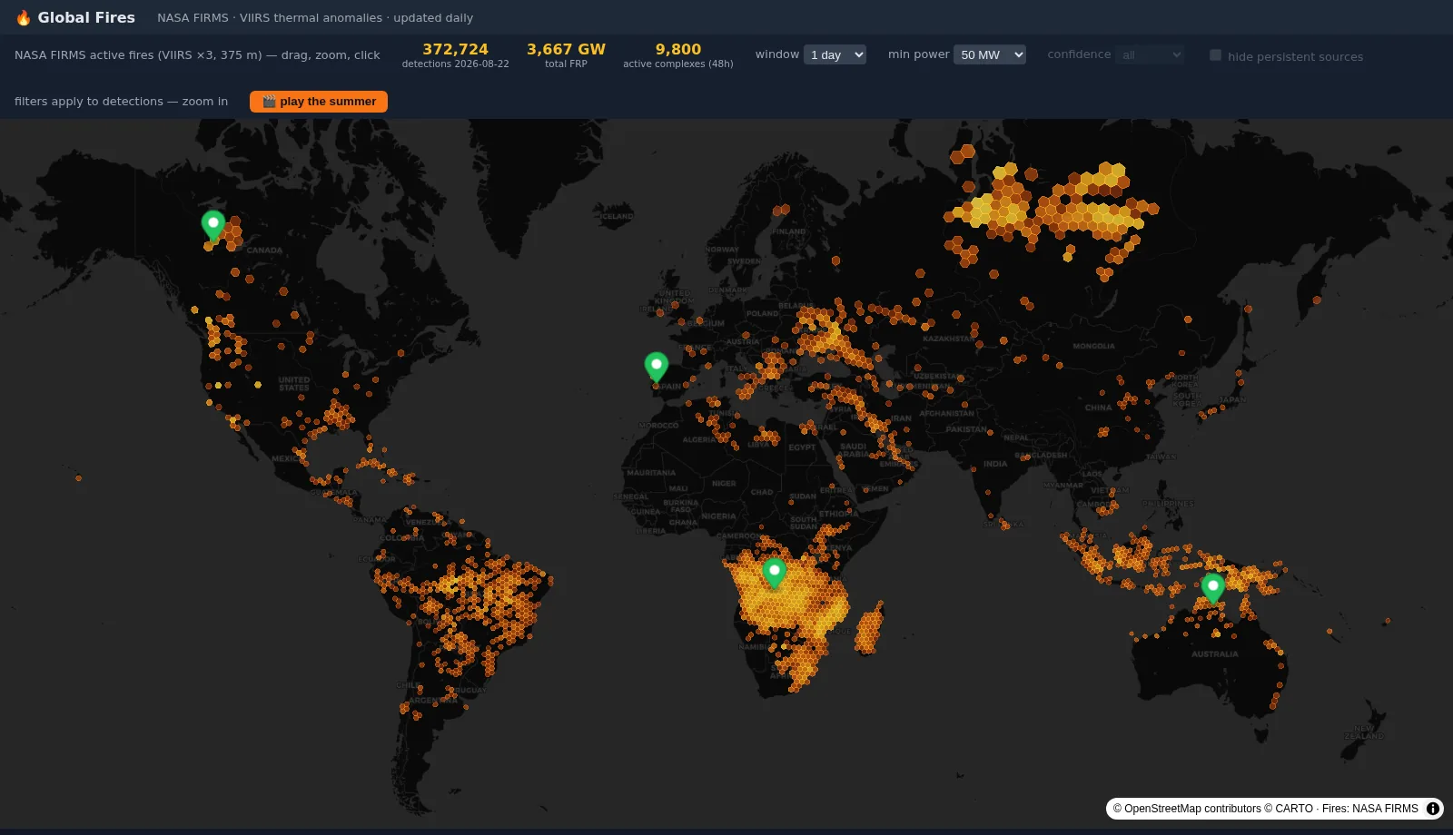
Every morning at 06:15 UTC a job wakes up, downloads the last three days of active-fire detections from NASA, and by 07:15 a dbt DAG has folded them into hexagons at three zoom levels. The result is a MapLibre globe: drag it, and you are looking at where the planet is burning.
The interesting parts of this project were not the parts I expected. The satellite data was easy. What shaped the architecture were three constraints: a platform that blocks outbound network calls, a data feed that rewrites its own past, and a projection problem that would have quietly invalidated every comparison I wanted to make.
This is one of two pipelines in Space Insights. Its counterpart, What a fire leaves behind, measures the same fires optically from Sentinel-2, and the two are built to check each other.
The constraint that shaped everything
The whole platform runs on Databricks Free Edition: serverless only, one workspace, zero cloud spend. That last part is a real design goal, not a brag: I wanted to prove the architecture stands up without a corporate account behind it.
Free Edition restricts serverless egress to an allowlist of trusted domains. NASA is not on it. So the most basic operation in the pipeline - GET a CSV from a public API, cannot happen inside the lakehouse.
Rather than fight that, I inverted it. The network-touching step runs outside Databricks as a scheduled GitHub Actions workflow that pushes into the workspace: files through the Files API, metadata through the SQL warehouse. I call these ground stations, and there are three of them: one for Copernicus Sentinel-2 imagery, one for Mars rover telemetry, and this one for fires.
Why this is not a hack
What the data actually is
NASA FIRMS publishes near-real-time detections from VIIRS, the imaging radiometer flying on Suomi-NPP, NOAA-20 and NOAA-21. Three separate satellites in three separate polar orbits, so pulling all three is not redundancy; it is more passes per day over the same ground.
Each row is one 375-metre pixel that the onboard algorithm flagged as anomalously hot, based on the ratio between two infrared channels:
latitude,longitude,bright_ti4,scan,track,acq_date,acq_time,
satellite,instrument,confidence,version,bright_ti5,frp,daynight
21.41485,-158.0162,337.92,0.48,0.4,2026-07-18,7,N,VIIRS,
n,2.0NRT,300.46,3.13,D
The field that matters most is frp, Fire Radiative Power, in megawatts. It is the energy release rate, and the best available proxy for how hard something is burning. It is what I weight by, colour by, and sort by throughout the stack.
An honesty problem worth naming
A feed that rewrites its own past
Near-real-time data is provisional. NASA restates recent detections as better geolocation becomes available, so yesterday's rows are not guaranteed to match what you fetched yesterday.
The obvious design (a watermark cursor, append everything newer than last time) is wrong here. It would accumulate stale duplicates of the same detection, each a slightly different version of the truth.
So the ingest is date-keyed replacement instead:
DELETE FROM firms_bronze.detections WHERE acq_date >= :min_date

INSERT INTO firms_bronze.detections
SELECT source, latitude, ..., current_timestamp()
FROM read_files('/Volumes/.../detections_20260815T061500.csv',
                format => 'csv', schemaHints => '...',
                mode => 'FAILFAST')
Fetch three days, delete those three days, re-insert them. No cursor table, no watermark, no state to corrupt. Three properties fall out for free: re-running is safe, NASA's revisions self-heal, and a missed run is repaired by the next one because the window is wider than the schedule.
Two smaller decisions in that snippet matter more than they look. mode => 'FAILFAST' means a malformed row aborts the entire insert rather than landing as nulls, and the ingest separately rejects any CSV whose header has drifted from the expected 14 columns. A schema change upstream should break my pipeline loudly, not quietly corrupt a year of history.
Three layers, three different jobs
Everything downstream of that insert is a medallion architecture - bronze, silver, gold, and the split is not ceremony. Each layer is allowed to do exactly one kind of work, which is what makes it possible to reason about where a bug can live.
- Bronze lands the data as it arrived, typed but otherwise unaltered, and fails loudly if it does not match expectations. No interpretation.
- Silver makes it trustworthy: deduplicated, correctly typed, enriched with the keys everything downstream joins on. Still one row per detection.
- Gold answers questions. Every model here exists because something in the UI asks for it.
Bronze onwards is entirely dbt, which matters for a reason beyond taste: three separate projects (fires, Sentinel-2, and Mars telemetry) share one dbt project, isolated by tag. The fires job runs dbt build --select tag:firms and touches nothing else.
What silver actually cleans
One model, detections_clean, doing four things.
First, deduplicate on the natural key. Bronze already guarantees no duplicates through delete-then-insert, so this is belt and braces - but it means the natural key holds regardless of how bronze was loaded, including by a future me doing a manual backfill at 11pm:
qualify row_number() over (
    partition by source, latitude, longitude,
                 acq_date, acq_time, satellite
    order by ingested_at desc
) = 1
Those six columns are what actually identify a detection: one satellite, one pixel, one overpass. ingested_at desc keeps the most recently loaded copy, which is the one reflecting NASA's latest revision.
Second, build a real timestamp. This is where the unpadded time field bites. NASA sends HHMM with leading zeros stripped, so a fire detected at seven minutes past midnight arrives as the string 7:
to_timestamp(
    concat(cast(acq_date as string), ' ', lpad(acq_time, 4, '0')),
    'yyyy-MM-dd HHmm'
) as acq_datetime
Without the lpad, every detection in the first ten hours of each day either fails to parse or lands at the wrong hour. It is a one-function fix, but the kind that produces a subtly wrong dashboard rather than an error.
Third, index into H3 at three resolutions. The next two sections are about why, because it is the most interesting decision in the pipeline.
Fourth, drop what nothing uses: scan and track geometry, instrument name, algorithm version.
What silver deliberately does not do
Why hexagons
A quarter-million points a day is too many to draw. They need aggregating, and the obvious way is to round the coordinates: GROUP BY round(lat, 1), round(lon, 1).
That would have quietly ruined the project.
Meridians converge toward the poles. A one-degree box covers about 12,300 km² at the equator and about 4,200 km² at 70°N. The regions I monitor span the Angola/DRC miombo belt at 10°S and the Northwest Territories boreal complex at 64°N, so “detections per cell” would mean something different in each place, and every comparison between the tropics and the boreal forest would be measuring the map projection instead of the fires.
H3 solves this. It tiles the globe with near-equal-area hexagons by subdividing an icosahedron and projecting onto the sphere. Sixteen resolutions; I index three of them:
| res | cells worldwide | avg area | roughly |
|---|---|---|---|
| 3 | 41,162 | 12,393 km² | a small country |
| 4 | 288,122 | 1,770 km² | a metro area |
| 5 | 2,016,842 | 253 km² | a large city |
Indexing is just bucketing: a continuous coordinate becomes a discrete cell ID, and a spatial question turns into string equality. No geometry library, no spatial join - GROUP BY h3_5 is an ordinary hash aggregation.
Hexagons buy a second property that squares cannot: uniform adjacency. Every hexagon has six neighbours, all equidistant. A square grid has four edge-neighbours and four corner-neighbours 1.41× further away, so “adjacent” is ambiguous, which matters the moment you try to cluster or model spread.
The 7% bug I nearly shipped
My silver table computes all three resolutions independently from the raw coordinate:
h3_h3tostring(h3_longlatash3(longitude, latitude, 3)) as h3_3,
h3_h3tostring(h3_longlatash3(longitude, latitude, 4)) as h3_4,
h3_h3tostring(h3_longlatash3(longitude, latitude, 5)) as h3_5
That looks wasteful. H3 is hierarchical (the cell IDs literally share a prefix) so surely you index once at the finest resolution and truncate to get the coarser ones?
No. Hexagons do not tile into hexagons. You cannot subdivide a hexagon into seven smaller hexagons cleanly; H3's children only approximately tile their parent, overlapping and gapping at the edges. Logical containment in the index is exact; geographic containment is not.
I measured it over 200,000 random points:
14,309 / 200,000  (7.15%)  of points land in a res-5 cell
whose res-4 parent differs from the point's
directly-assigned res-4 cell
Rolling up instead of re-indexing would have misattributed about 7% of detections to the wrong coarse hexagon, and not randomly. The errors concentrate at cell boundaries, which is exactly where a large fire complex straddles two cells and where you most want the count to be right.
The general lesson
What gold actually computes
Five models, all dbt, all rebuilt every morning, and rebuilt with dbt build rather than dbt run, which is the difference between running the models and running the models plus their tests. Grain uniqueness and not-null assertions execute on every daily run, and a failure fails the job. Silently producing a duplicated hexagon is not a failure mode I want to discover from the map looking wrong.
fires_daily_h3: the hexagons
Three resolutions stacked into one table by a Jinja loop that unions three aggregations of the same source:
{% for res in [3, 4, 5] %}
select {{ res }} as h3_res, h3_{{ res }} as h3_cell, acq_date,
       count(*) as n_detections, sum(frp) as frp_sum,
       sum(case when confidence = 'h' then 1 else 0 end) as n_high_conf
from {{ ref('detections_clean') }}
group by h3_{{ res }}, acq_date
{% if not loop.last %}union all{% endif %}
{% endfor %}
The two Jinja expressions do different things and it is worth reading them slowly: {{ res }} emits a literal (3, 4 or 5), while h3_{{ res }} emits a column name. So the resolution tag has three distinct values across the whole table, while the cell column holds tens of thousands.
Stacking them means the client swaps aggregation level on zoom with one query shape and a changed integer, rather than three different endpoints. The grain (resolution, cell, date) is enforced by a uniqueness test, so the union cannot quietly produce overlapping rows.
fires_daily_stats: the headline numbers
The same aggregation with the spatial dimension removed: one row per day, global totals, feeding the counters above the map.
It looks redundant: surely you can sum the hexagons? Almost, but not quite, and the exception is a nice reminder that not every aggregate is additive. Detection counts and total fire power roll up fine. The number of distinct satellites contributing does not: summing per-cell distinct counts would count Suomi-NPP once per hexagon it appears in. Distinct counts have to be computed at the grain you want to read them at.
active_fires: the one with actual logic in it
“Fire complexes” over the trailing 48 hours: coarse cells with at least three detections, ranked by intensity. Three decisions in here I would defend in a review.
The window is anchored to the data, not the clock:
with window_bounds as (
    select max(acq_datetime) as latest from {{ ref('detections_clean') }}
)
Using current_timestamp() would have been the obvious move and it would have been wrong twice over. Wrong for testing, because the model produces different output depending on when you run it. And wrong operationally: if ingest fails one morning, a wall-clock window silently slides past all the data and the map goes empty, which looks like “no fires on Earth today” rather than “the pipeline is broken”. Anchored to the newest row, it just shows slightly older data and stays obviously alive.
The centroid is weighted by fire power:
sum(latitude * frp) / sum(frp)  as centroid_lat,
sum(longitude * frp) / sum(frp) as centroid_lon
A plain average puts the marker in the geometric middle of the detections, which for a long fire front is often somewhere nothing is burning. Weighting by power drags it toward the hottest part, where you would actually send an aircraft. This is also why the model filters to rows with positive fire power: the division needs a non-zero denominator.
The trend is a ratio of consecutive 24-hour halves:
sum(case when acq_datetime > latest - interval 24 hours
         then frp else 0 end)
  / nullif(sum(case when acq_datetime <= latest - interval 24 hours
                    then frp end), 0) as frp_trend
Above 1 means growing, below means dying down. The nullif matters more than it looks: a complex with no activity in the previous period would divide by zero, and the honest answer there is not “infinite growth” but null, a brand-new fire with no baseline to compare against. Encoding “I cannot know this” distinctly from a number is most of what makes a metric trustworthy.
Finally a noise floor of at least three detections. One hot pixel is not a fire complex; it is usually a factory.
detections_recent: a view, for an unglamorous reason
Last seven days of individual detections, unaggregated. It exists in gold purely because of permissions: the app's service principal is granted read access to the gold schema only, and Unity Catalog views execute with their owner's privileges. The view lets the app read silver-grade data without ever holding a grant on silver. Not a modelling decision at all, but an access-control one wearing a modelling costume.
s2_firms_agreement: checking one pipeline against another
The one I find most satisfying. My Sentinel-2 pipeline detects burn scars optically, by measuring how vegetation reflectance changed between two dates. FIRMS detects heat. Those are genuinely independent physical signals from different satellites, so where they agree, confidence goes up a lot.
This view joins them: FIRMS points falling inside a monitored region are mapped onto the Sentinel-2 analysis grid and matched to burn-scar cells within three days. It is a view rather than a table because the two pipelines rebuild an hour apart; a table would always be showing one run of stale agreement.
The other side of that join, how a burn scar is measured in the first place and why the change matters rather than the reflectance, is its own write-up: What a fire leaves behind.
Sending IDs instead of shapes
One detail I am fond of. The API never sends hexagon geometry to the browser. It sends the cell ID and two numbers:
{ "h3": "8446483ffffffff", "n": 214, "frp": 8231.4 }The client reconstructs the polygon with cellToBoundary() from h3-js. A hexagon as GeoJSON is seven coordinate pairs, around 120 bytes. As an H3 ID it is 15 characters. Across tens of thousands of cells that is most of an order of magnitude of bandwidth, and the client-side cost is a function call that was already loaded.
The string form is not cosmetic either. H3 IDs are 64-bit integers, and JSON has no int64 - 591208020730445823 exceeds JavaScript's safe integer range and would silently lose precision in transit. The hex string is the only safe wire format.
The demo has no backend at all
There is a constraint I did not see coming until I tried to share this. Databricks Apps cannot be made public: anonymous access and SSO bypass are unsupported, and the free tier has no identity provider to enrol outside viewers through. A link to the running app shows every visitor a login wall they have no way past.
So the globe is republished every morning as a static site instead. Worth being precise about what that means, because the word is slippery: the frontend was always static, a compiled bundle of HTML, CSS and JavaScript. What changed is that there is no longer a server process sitting next to those files. Previously one uvicorn process served both the bundle and the /api/* routes that queried the warehouse. Now there is a file host and nothing else.
That single change has a sharp consequence: nothing can answer a question at request time, so every answer has to exist as a file before anyone asks it.
For the hexagons that is easy. The UI only ever asks for three resolutions across three time windows, so there are nine possible answers and I pre-render all nine to JSON. For individual detections it is not easy at all, because the question is “what is inside this box” and every pan and zoom invents a new box. You cannot enumerate those.
Changing the question
The fix is PMTiles, and what I like about it is that it does not answer the hard question - it replaces it with an easy one.
Map data is conventionally cut into tiles: a grid at each zoom level, each square stored separately. That normally means hundreds of thousands of files and a tile server to route between them. PMTiles packs the whole pyramid into one file with an index at the front. The client reads the index, works out that the tile it wants sits at a particular byte offset, and asks for exactly those bytes:
GET /fires.pmtiles
Range: bytes=4182000-4190999
That is an ordinary HTTP range request, the same mechanism that lets you scrub into the middle of a video without downloading it. “Which detections are in this box?” requires understanding the data. “Give me these bytes” requires understanding nothing, which is precisely why a dumb file host can serve it.
The version with no server is the better one
One wrinkle worth recording, since I got it wrong first. I assumed the whole thing could sit on Cloudflare Pages. It cannot: Pages does not serve range requests correctly and caps files at 25 MiB, and the archive is larger than that. The tiles live on R2 (object storage, range requests supported, no egress fees) while Pages serves the bundle and the small JSON. Two hosts, still nothing to operate, still zero a month.
What the data actually says
Two months of archive, 1 July to 22 August 2026, is 11.4 million detections across 176 countries. That is enough to answer a few questions the news does not, and the answers were not what I expected.
The first is that the planet burns most in places that never make a headline.
| Country | Detections | Share |
|---|---|---|
| DR Congo | 1.8M | 16% |
| Angola | 1.7M | 15% |
| Russia | 1.4M | 12% |
| Zambia | 1.2M | 11% |
| Canada | 0.97M | 9% |
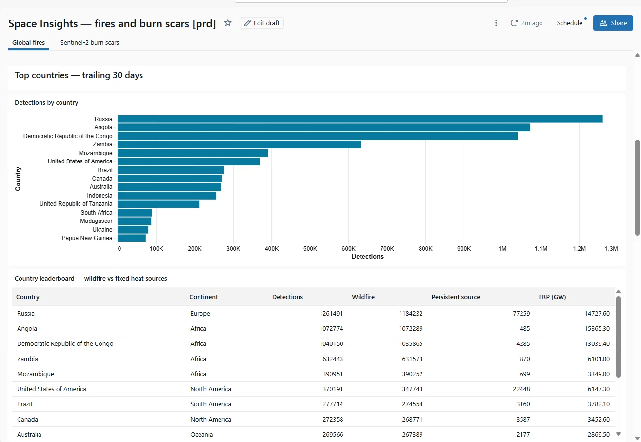
Southern-African savanna dwarfs everything else. Three countries account for roughly two fifths of every thermal detection on Earth this summer, and almost none of it reaches a European news cycle. The honest caveat matters as much as the number: most of that signal is seasonal savanna and agricultural burning, a fire regime that has run on the same annual cycle for a very long time. It is not the same phenomenon as a Mediterranean crown fire, and reporting it as though it were would be its own kind of distortion. What the count measures is heat, not catastrophe.
Within the EU, Spain came out on top with 35,575 wildfire detections, and nearly twice the radiative power of Portugal and France combined. Europe barely registers globally while dominating the coverage, which is a reasonable thing for coverage to do and a terrible thing for a dataset to do.
A lot of “fire” is not fire
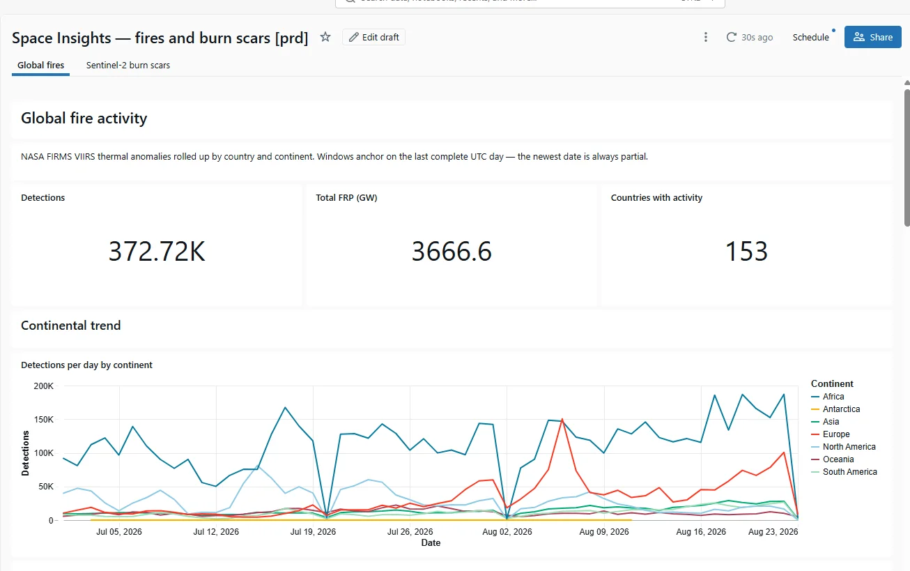
The busiest single day in the archive was 6 August 2026, at 374,310 detections radiating a combined 5.4 million megawatts. That is the number the replay animation is climbing toward.
What I would change
The honest weakness is retention. Bronze never prunes, and every silver and gold model is a full rebuild, so each morning re-aggregates the entire history. At current volume that is fine. After a year it is 90 million rows being re-scanned daily to recompute numbers that have not changed since they landed.
The fix is not exotic: incremental models keyed on acquisition date with a lookback matching the revision window, plus a retention policy on bronze. I have deliberately not built it yet, because the pipeline that exists is correct and the one I would replace it with is merely faster, and I would rather have a stated tradeoff than a premature optimisation.
The second weakness is a fragile join. A view cross-validates my Sentinel-2 burn-scar detections against FIRMS hotspots by recomputing my analysis-grid cell IDs in SQL, duplicating a formula that lives in Python. Nothing enforces that the two stay in sync. If I change the grid, the view produces wrong joins silently rather than failing. A shared fixture asserting both implementations agree is the real fix; a code comment is what is there now.
The third is not a weakness so much as a ceiling. Precomputing every answer works because the questions are few and known: nine hex slices and a fixed tile pyramid. It stops working the moment someone wants to ask something I did not anticipate: filter by satellite, compare two arbitrary date ranges, draw their own region of interest. That is the point at which I would put the API back, on Cloud Run with a real database and a cache in front, and keep the tiles for the bulk geometry. I would rather arrive there because a question demanded it than start there because it felt more like architecture.
The stack
- Source: NASA FIRMS area API, three VIIRS NRT feeds, CSV.
- Ingest: Python on GitHub Actions cron, the ground station.
- Lakehouse: Databricks Free Edition: Unity Catalog, Delta, UC Volumes, serverless SQL.
- Transform: dbt, tag-isolated so three projects share one dbt project without colliding. H3 via native Databricks SQL functions.
- Serving: React 19 and MapLibre GL globe projection, h3-js for client-side geometry. FastAPI behind it in the workspace app; nothing behind it in the public one.
- Publishing: tippecanoe builds the tile archive; Cloudflare Pages serves the bundle, R2 serves the tiles. Republished daily by a scheduled workflow.
- Infrastructure: Terraform for workspace objects, Databricks Asset Bundles for jobs and apps. No click-ops.
Total running cost: zero. That constraint produced better engineering than a budget would have. Every architectural decision had to be justified against a platform that said no a lot.